Why Customer Lifetime Value Forecasting Is the Metric Your Revenue Strategy Can't Ignore
Customer lifetime value forecasting is the process of predicting how much revenue a customer will generate over their relationship with your business — so you can make smarter decisions about acquisition, retention, and budget allocation before the money is spent.
Quick answer: Here are the three main approaches to CLV forecasting:
| Approach | Best For | Key Tool |
|---|---|---|
| Heuristic | Fast estimates, early-stage data | ARPU ÷ Churn Rate |
| Probabilistic (BG/NBD + Gamma-Gamma) | Non-contractual repeat-purchase businesses | Lifetimes / PyMC-Marketing |
| Machine Learning | Large datasets, complex behavior patterns | Random Forest, XGBoost, dRNN |
Most finance and RevOps teams treat CLV as a lagging metric — something you calculate after the fact. That's a problem.
By the time you know a customer's lifetime value, you've already made every decision that determined it: how much you paid to acquire them, which segment you put them in, whether you reached out before they churned.
The better approach is to forecast CLV forward — using transaction history to predict future value at the individual customer level.
And the stakes are real. A 5% reduction in annual churn (say, from 15% to 10%) can raise average LTV by 20% — from $2,000 to $2,400. That's not a rounding error. That's a strategic lever.
For a SaaS or subscription business, this matters even more. Your revenue isn't transactional — it compounds. Knowing which customers are likely to expand, stay flat, or churn in the next 90 days changes how you deploy your entire go-to-market budget.
This guide walks through the models and heuristics that actually work, how to choose between them, and how to put the outputs to use.
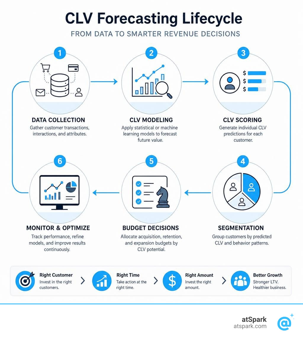
Demystifying Customer Lifetime Value: Core Concepts and Common Myths
To build a reliable forecasting engine, we must first clear away the myths that plague standard customer lifetime value calculations.
A common pitfall is treating CLV as simple historical revenue. If a customer spent $500 last year, is their CLV $500? Absolutely not. Real CLV represents the net present value of the future cash flows expected from a customer relationship. That means we must shift our focus from top-line revenue to profit margin, and apply a discount rate to account for the time value of money.

When evaluating long-term profitability, we must balance What is Customer Lifetime Value (LTV)? against the cost of acquiring that customer. A healthy business benchmark targets a LTV:CAC Ratio of 3x to 5x or greater. If your ratio drops below 3x, your acquisition strategy is likely destroying business value.
Let us break down the three most common myths in CLV modeling:
- Myth 1: CLV means lifetime revenue. Calculating CLV using pure revenue leads to overspending on acquisition. To get a true picture, you must multiply projected revenue by your gross margin, and then discount those future cash flows.
- Myth 2: The "lifetime" is infinite. We do not model customer relationships over a literal lifetime. In practical business applications, we forecast over a fixed horizon — typically 12, 24, or 36 months — aligned with our strategic planning cycles.
- Myth 3: Future value is the same as calendar value. This is a frequent point of confusion. Calendar value projects the total revenue generated by a business during a specific period (which includes revenue from future, yet-to-be-acquired customers). CLV, on the other hand, isolates the future residual value of your existing cohort, assuming no new acquisitions.
Understanding your Customer Churn Rate is critical to correcting these assumptions. If your churn rate is high, your projected customer lifespan shrinks, dragging your forecasted CLV down with it.
Three Approaches to Customer Lifetime Value Forecasting
There is no one-size-fits-all model for predicting customer value. The right choice depends on your business model, data maturity, and strategic goals.
We categorize forecasting models into three distinct methodologies:
- Heuristic Models: These are simple, rule-based formulas that use aggregate business metrics (like average order value and overall churn) to establish a baseline. They are excellent for quick, company-wide sanity checks but fail to capture individual customer differences.
- Probabilistic Models: These statistical frameworks, such as the "Buy-Till-You-Die" (BTYD) family, model purchase frequency and churn probability as independent probability distributions. They are highly effective for non-contractual retail settings where customers "churn silently" without telling you.
- Machine Learning & Deep Learning: These supervised models use algorithms like Random Forests, XGBoost, or Recurrent Neural Networks (RNNs) to find complex, non-linear patterns in customer behavior. They require rich, clean datasets but deliver high precision.
For teams looking to dive deeper into programmatic execution, resources like 4.2 Customer Lifetime Value Modeling – Marketing Science in Python offer excellent starting points for building custom probabilistic models.
| Metric | Heuristic Approach | Probabilistic (BG/NBD) | Machine Learning |
|---|---|---|---|
| Data Required | Aggregate ARPU & Churn | RFM-T transaction history | Multi-source behavioral data |
| Granularity | Cohort or Segment level | Individual customer level | Individual customer level |
| Implementation | Spreadsheet (Minutes) | Python / R libraries (Days) | Custom ML pipeline (Weeks) |
| Key Advantage | Fast and easy to explain | Great for silent churn | Highly accurate with rich data |
How to Prepare, Split, and Model Transaction Data
Before running any predictive algorithm, you must clean and structure your transaction data. Raw billing logs are messy; they contain negative values from refunds, zero-dollar promotional credits, and timezone discrepancies.
To prepare your dataset, you should remove all non-positive transactions and normalize your timestamps. For a step-by-step breakdown of enterprise data requirements, review the standards in ci-docs/data/predict-customer-lifetime-value.md.
Once your data is clean, you must summarize individual purchase histories into four core statistical features, known as RFM-T:
- Recency: The time elapsed between a customer's first purchase and their most recent purchase.
- Frequency: The number of repeat purchases a customer has made (excluding the very first order).
- Monetary Value: The average order value of those repeat transactions.
- Tenure (T): The total age of the customer in your system, measured from their first purchase to the end of your observation period.
To train and validate your model without cheating, you must split your historical data carefully to avoid temporal leakage (where the model accidentally looks into the future during training).
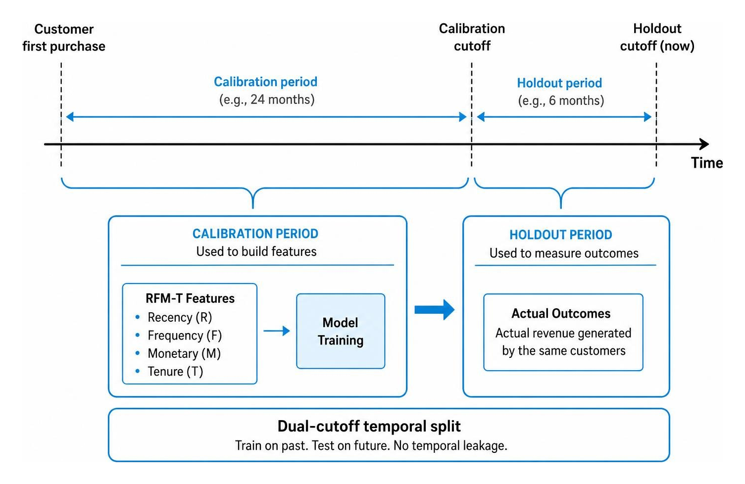
Instead of a simple random split, we use a dual-cutoff temporal split:
- Calibration Period: A historical window (e.g., 24 months) used to calculate the RFM-T features for each customer.
- Holdout Period: A subsequent window (e.g., 6 months) used to measure the actual revenue generated by those same customers.
By training your model on the calibration features and comparing its predictions against the actual holdout outcomes, you can objectively measure its real-world performance.
How to Calculate CLV Using the Heuristic Method
The heuristic method is the easiest way to estimate customer value. It relies on two main metrics: Average Revenue Per User (ARPU) and your churn rate.
The baseline formula is straightforward:
- CLV = ARPU ÷ Churn Rate
If your average customer generates $100 per month and your monthly churn rate is 5%, the estimated lifespan is 20 months (1 ÷ 0.05), yielding a baseline CLV of $2,000.
For long-term financial planning, you should also apply a discount rate (such as your weighted average cost of capital) to find the net present value of those future months.
To run these calculations quickly, you can use our interactive LTV Calculator to test different scenarios. That tracking these figures requires a solid grasp of your SaaS Customer Retention Metrics.
While heuristics are helpful for high-level budgeting, they assume every customer is identical. If 10% of your users contribute to 80% of your revenue, a blended average will misrepresent both your highest and lowest value segments.
Probabilistic Modeling: BG/NBD and Gamma-Gamma for Customer Lifetime Value Forecasting
To solve the limitations of simple averages in non-contractual business settings, data scientists use the Beta Geometric/Negative Binomial Distribution (BG/NBD) model combined with the Gamma-Gamma submodel. This is often called the "Buy-Till-You-Die" framework.
The model splits the customer journey into two independent processes:
- The Transaction Process (BG/NBD): This determines when and how often a customer will buy. It assumes that while active, a customer's transactions follow a Poisson process. It also assumes that after any transaction, the customer has a certain probability of dropping out (churning silently), modeled by a Beta distribution.
- The Monetary Value Process (Gamma-Gamma): This determines the economic value of those future transactions. It assumes that monetary value is distributed according to a Gamma-Gamma structure, which acts as a shrinkage estimator — pulling customers with very few transactions toward the population average to avoid wild, unrealistic predictions.
A key requirement of this framework is that transaction frequency and monetary value must be independent. For a deeper look at how these components combine into discounted cash flows, see the technical breakdown in Predictive CLTV Modeling.
Machine Learning and Deep Learning for Customer Lifetime Value Forecasting
While probabilistic models are highly interpretable, supervised machine learning can capture complex, non-linear relationships that statistical models miss.
By training a Random Forest Regressor or an XGBoost model on your RFM-T features alongside demographic and behavioral data (such as website visits or email clicks), you can significantly improve forecasting accuracy.
In retail transaction tests, the BG/NBD model can deviate from actual values, yielding a Mean Absolute Error (MAE) of $954 against a mean true 3-month CLV of $1,538. Switching to a Random Forest Regressor on the exact same features can reduce that MAE to $912.
For enterprise platforms with massive datasets, deep learning offers even greater precision. Researchers have developed Recurrent Neural Networks (RNNs) using dilated RNN (dRNN) cells to handle long-term temporal dependencies. These models use feature embeddings to map categorical variables (like location or acquisition channel) into continuous vectors, outperforming traditional models across long-term horizons.
To explore the academic validation of these neural networks, read Predicting Customer Lifetime Value Using Recurrent Neural Net.
Evaluating Model Performance Against Actual Future Revenue
You cannot manage what you do not measure. To validate your CLV forecasts, you must compare your model's predictions against the actual revenue generated during your holdout period.
The most common evaluation metrics include:
- Mean Absolute Error (MAE): Measures the average absolute difference between predicted and actual values.
- Root Mean Squared Error (RMSE): Penalizes larger errors more heavily, making it useful for identifying extreme outliers.
- Adjusted Symmetric Mean Absolute Percentage Error (aSMAPE): Prevents skewed error rates when dealing with customers who had zero transactions in the holdout period.
When evaluating machine learning approaches, we must also look out for temporal leakage. For a detailed guide on configuring honest evaluation pipelines, consult Customer Lifetime Value (CLTV) Forecasting.
Frequently Asked Questions about CLV Forecasting
How can businesses use CLV predictions for customer segmentation and marketing strategy?
Predictive CLV changes how you run your go-to-market campaigns. Instead of treating all customers the same, you can segment them by their predicted future value:
- VIP Targeting: Focus your high-touch loyalty programs, exclusive offers, and priority customer service on the top 10% of customers who are predicted to drive the majority of your future revenue.
- CRM Churn Alerts: Set up automated triggers in your CRM when a customer's probability of being active, P(alive), drops rapidly (for instance, a 30-point drop within 30 days). This allows your customer success team to reach out before the customer is gone for good.
- Smart Acquisition (CPA Ceilings): Set your maximum Customer Acquisition Cost (CAC) as a fraction of your predicted profit CLV. This prevents you from overspending on cheap, high-churn segments while allowing you to bid more aggressively for high-value cohorts.
What are the limitations of standard CLV models for new customers, and how does survival analysis help?
Standard CLV models suffer from a cold start problem. Because they rely on historical transaction frequency and recency, they cannot reliably predict the value of a brand-new customer who has only made one purchase.
To solve this, we can use survival analysis. Instead of waiting for a customer to compile a long transaction history, survival analysis models the "hazard rate" (the probability of churn occurring at any given tenure) based on early behavioral signals and demographic data. This allows us to estimate a customer's survival curve and project their lifespan from day one.
How does an AI-driven CLV model compare to a simple baseline model?
A standard mathematical baseline model calculates CLV by multiplying a customer's average historical monthly spend by your overall retention rate.
An AI-driven model, however, looks at individual behavioral changes, customer profile attributes, and engagement history. In enterprise testing, AI models are graded on how much better they perform compared to this baseline. An "A" grade represents a 5% or greater improvement in accurately predicting high-value customers.
To learn how to set up and run these comparative models, check out Predict customer lifetime value (CLV) - Dynamics 365 Customer Insights | Microsoft Learn.
Conclusion
Building and maintaining predictive CLV models used to require a dedicated team of data scientists and complex engineering pipelines. But today, unified data makes these insights accessible to everyone.
At atSpark, we help SaaS companies bypass the complexity. Our AI-powered analytics platform unifies your billing, CRM, and subscription data into a single source of truth. Instead of writing SQL queries or building custom Python pipelines, you can ask plain-English questions and get instant, beautifully formatted charts and tables.
By connecting your customer touchpoints, atSpark gives you the clarity you need to make fast, data-driven decisions that grow your business. Learn more about ARR tracking and see how conversational analytics can transform your growth strategy.